Generative models encode data and behavior in high-dimensional representation spaces, where surprisingly simple vector operations can often produce meaningful changes in model outputs. This article develops an intuitive geometric view of model steering through three basic ingredients: a base point, a direction, and a step size. Using a determinstic generative model (StyleGAN2)
King − Man + Woman ≈ Queen
Many people have encountered the famous example of king − man + woman ≈ queen observed in word embedding models. Although surprisingly simple and intuitive, this example demonstrates an important idea: relationships become directions in a high-dimensional space. Arithmetic on these vectors does not merely manipulate numbers—it manipulates meaning. This observation provides an intuitive starting point for understanding how similar vector operations can steer modern generative AI systems.
Generative Models Are Everywhere
Today, generative AI has become a foundational technology across many domains. Large language models (LLM)
generate text and code
Steering Model Outputs
As generative models become increasingly capable, an important question is no longer whether they can generate
content, but whether we can reliably control what they generate. Activation steering has emerged as a lightweight
mechanism for influencing a model's behavior without retraining
it
Different models shape this world differently. StyleGAN2 transforms a random vector into an intermediate style
code before generating an image
Latent Spaces: Internal Representations of Data
To understand how steering works, we first need to understand latent spaces. In image generator models such as
StyleGAN2
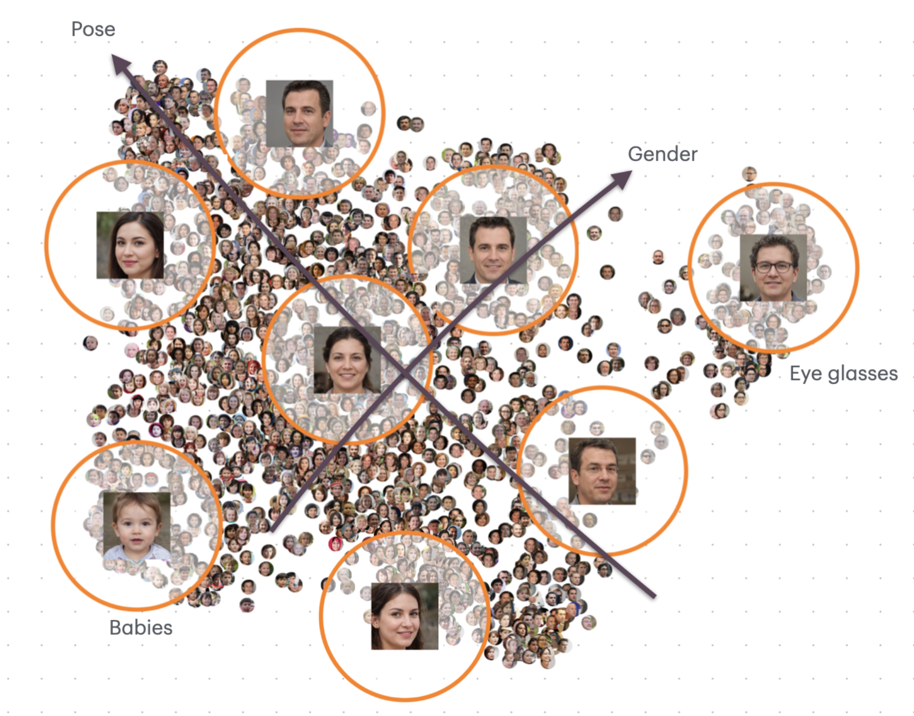
Generative model is composed of a seuqence of computation blocks, transforming input latent code (e.g., samples from a gaussian distribution) into intermediate/latent representations. By carefully choosing which latent space we work on for manipulation/steering, we are able to plot a sensible map of the entire latent landscape. As an example, here we use StyleGAN2's 32x32 convolutional block output, average downsampled to 5x5 feature maps, and use UMAP to reduce the 5x5x512 dimensional vectors to 2D. below we show a couple of semantically meaning directions we found in this generative landscape.
Three Ingredients for Navigation
Where to Begin, Which Direction to Take, and How Far to Travel
The math behind many steering techniques is remarkably simple. Starting from the latent vector of one example, we add or subtract another vector representing a semantic direction. These operations often produce smooth, meaningful transformations despite involving nothing more than elementary linear algebra. In this session we explain the contextural meaning behind adding and subtracting vectors in the latent space. And show how it behaves in real-world datasets and generative models.
The Base: Where Do We Start?
As with any journey across a map, we first have to decide where it begins. And in everyday life we rarely name that starting point by its coordinates. Latitude and longitude are precise and useful, but they are not how people actually navigate a place; we reach instead for landmarks — familiar checkpoints, and positions described relative to them.
Latent space works the same way. Its landmarks are the sample points the dataset already gives us, and each one
also has an exact address: the high-dimensional coordinates that play the role of latitude and longitude. So a
journey begins at some sample $z_i$, written as the vector
The Direction \vec{d} : Which Way Do We Go Next?
The direction determines how a base point can move or change in the generative model’s latent space along the entire path way of the movement. In general, such directions can be defined in so many ways, as long as it defines a vector field over the generative latent space. For example, it can be derived from local model geometry using a good basis obtained from a Jacobian matrix. A much simpler and computationally cheaper alternative, however, is to define them through contrastive pairs.
Given two groups of examples representing opposite concepts (e.g., short hair, long hair), we can compute the difference between their average latent representations. This difference captures the features that distinguish one group from the other and turns that contrast into an actionable direction of change. Moving along this direction can then steer a new base point toward one concept or the other.
As a simple example, a direction can be defined by subtracting two endpoints: an example representing the desired destination minus an example representing the opposite concept. In this case, the direction is specified using only two examples.
More generally, a direction can also be defined as the difference between the averages of two groups, or as the average of the differences between matched positive–negative pairs.
The Step Size \alpha : How Far Should We Go?
Once we know which direction to move, the next question is how far to go. The step size controls the magnitude,
or strength, of the change applied to the base point. A small step produces a subtle change, while a larger step
pushes the result farther along the chosen direction. Let
Here,
Example: Adjusting facial features
We use faces to demonstrate the basic idea of vector arithmetic in generative models. Here, we project the high-dimensional latent codes of generated examples onto a 2D map using dimensionality reduction (UMAP
Note that although the underlying algebra is entirely linear — a direction defined by a contrastive pair and applied to a base point forms a parallelogram in the original latent space — the same geometry does not necessarily appear as a parallelogram in the interface. UMAP is a nonlinear projection and therefore does not preserve this linear structure exactly in 2D.
The examples above illustrate how simple vector operations can produce meaningful semantic changes, along with several interesting and sometimes unexpected behaviors. They also demonstrate how a map-based interface can support multiple stages of steering: browsing the latent space, selecting examples to define directions, and locally refining those directions through interpolation.
As we have already seen, dimensionality reduction allows us to project samples from a high-dimensional latent space onto a 2D map and use the generative model to explore the resulting landscape. In these examples, distinct regions correspond to faces with different characteristics. However, no 2D projection can faithfully preserve all of the information and structure in a high-dimensional space. This raises a broader question: how can we design an interface that supports effective navigation and control directly within such a complex latent space?
Towards a Unified Model Steering Interface
The examples presented so far rely on a way of hand picking semantic directions one at a time. To make these operations more intuitive and efficient, so that users can freely explore the gerative capacity of a model, we envision an interface for exploring vector arithmetic in such models. Rather than exposing users directly to high-dimensional vectors or requiring them to combine directions through conventional sliders, interface can provide intuitive ways to define semantic directions, visualize interpolation paths, and manipulate latent representations through direct visual interaction. The goal is to make model steering feel more like navigating a map and mixing colors on a palette, allowing users to explore, combine, and refine semantic transformations without requiring expertise in machine learning.
Local Semantic Mixing through Interpolation Interface
As we have seen, a global semantic direction can be defined by taking the difference between two sets of examples. Although surprisingly effective, such directions remain only approximations and can easily become entangled with correlated attributes. For instance, in the earlier example, the direction intended to represent gender was also correlated with hair length. This problem is especially pronounced when the positive and negative groups contain only a small number of examples, since the resulting vector may capture several correlated variations at once rather than isolating the intended semantic concept. Ideally, we would like to find two points that differ along only a single semantic feature, so that the vector connecting them represents a fully disentangled direction: moving along it changes the intended attribute while leaving other features unchanged. In practice, however, such perfectly matched pairs are difficult to find directly in the data. This motivates local steering and refinement methods, which adjust or interpolate nearby examples according to the local geometry of the latent space in order to cancel unwanted correlated variations and better isolate the semantic factor of interest.
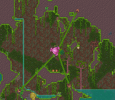
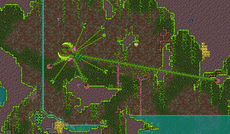
A key idea behind local mixing is that the three components involved in vector arithmetic—1) the base point, 2) the positive point, and 3) the negative point—do not need to correspond to individual examples. Instead, each can be defined as an interpolated point formed by taking a weighted average of several nearby examples. One way to think about this interaction is as a color-mixing palette: moving reference examples, like different paints, closer to the central interpolation point gives them greater weight in the resulting mixture. Another analogy is an octopus pulling on a collection of marbles: examples closer to the control point exert a stronger influence, while more distant examples contribute less.
Specifically, we combine the latent codes of the reference samples, $z_i$, using a weighted linear combination:
Choice of weight functions
In principle, the weighting function can be any monotonically decreasing function of distance: nearby examples should contribute more, while distant examples should contribute less. In the octopus figure, we experiment these two examples. The first uses an inverse-distance weighting scheme, in which each weight is proportional to $1/d$, where $d$ is the distance to the control point. The second uses a smooth, step-down weighting function with finite support, so that the contribution gradually decreases with distance and becomes zero beyond a specified cutoff radius.
Alongside those two, the figures offer a third weighting function that sits between them:
The three differ first in how sparse the resulting mixture is. Inverse distance never reaches zero, so every sample contributes something at every position: wherever the control point is placed, the whole reference set is in the average, and no single sample ever holds much of it. Both compactly supported functions instead produce a genuinely local mixture — a handful of nearby samples, with the nearest one holding most of the weight — and both figures show the same ordering. A dense mixture is a better-estimated local mean and changes gradually as the control point moves; a sparse one commits to a few samples, rewrites much more of its composition for the same movement, and can empty out altogether if the control point strays far enough from every sample. That is the trade the cutoff radius controls.
Sparsity, though, is nearly the same for the two compactly supported functions. What separates them is where along the distance axis each one discriminates — how sharply a weight responds to a given proportional change in distance. For inverse distance that response is the same everywhere, which is also why its normalised weights are invariant to a uniform rescaling of the layout: there is no radius to choose, and zooming the map changes nothing. The smooth step-down is very nearly flat close in, treating everything well inside the cutoff as almost interchangeable and spending essentially all of its discrimination near the rim, where it falls away very steeply. The logarithmic function spreads the same total falloff far more evenly across the range, rising from gentle near the centre to steep near the cutoff and passing through inverse distance's constant response somewhere in the middle. So over the inner part of its support, where the step-down barely distinguishes one neighbour from another, the logarithm is already separating them.
Read as interface behaviour, this is a choice about how much of the neighbourhood a single control point should speak for. Inverse distance gives a broad, well-averaged base point that moves slowly and is never entirely free of distant samples — useful when a stable local mean is wanted, less so when the target is a specific pocket of the space. The smooth step-down gives a strictly local mixture with a soft boundary and a nearly uniform interior, which behaves much like a smooth $k$-nearest-neighbour average. The logarithmic function keeps that locality but restores a preference for the nearest sample throughout the support, so the mixture stays anchored to whatever the control point is closest to while still borrowing from its neighbours — a middle ground for the case where the intended contrast is carried by one example and refined by the rest.
The interface therefore behaves partially like what PromptPaint
An important consequence of this interface is that a simple 2D manipulation induces a coordinated mixture of many high-dimensional latent vectors. The user therefore acts in an intuitive 2D space, while the actual navigation takes place in the model’s much higher-dimensional latent space. This differs from a conventional slider, which typically moves a point along a single predefined direction. Here, moving $z$ changes its relative distance to multiple examples at once, continuously adjusting their contributions to the mixture. The color-mixing analogy captures this behavior particularly well: rather than specifying how far to move along one fixed axis, the user controls the relative influence of several examples simultaneously, much like changing a color by varying the proportions of multiple paints.
neighborhood layout around the mixing point also plays an important role, in determining what subsupace is reachable from the interface.
Global browsing through high dimensional latent space
Taking the idea of interpolation to a global scale, we can support global browsing by sweeping across a 2D projection of the latent space and continuously interpolating among nearby samples using the local mixing method described below. This process effectively lifts movement in the 2D interface back into the high-dimensional latent space, producing a continuous surface of interpolated latent states. More precisely, the interface defines a 2D parameterized surface within the high-dimensional space. Compared with a linear projection, which is restricted to a single linear subspace, this approach can trace a richer and more diverse region of the latent landscape, allowing users to explore complex variations through simple two-dimensional navigation.
Directional steering through contrastive pairs
As we have seen, a steering direction can be defined by contrasting two sets of examples: a positive group and a negative group. The difference between their aggregated latent representations determines a semantic direction in the latent space. The global browsing interface can therefore serve not only as a tool for exploration, but also as an interactive mechanism for selecting and constructing these contrastive groups directly from the data. By browsing the latent landscape and identifying representative regions, users can define steering directions visually rather than specifying them through individual examples or predefined labels.
Putting things together
Towards a Unified Interface for Generative Model Output Manipulation
Putting these ideas together, interpolation among the mapped sample points allows us to navigate a simplicial complex defined by those samples in the latent space. Importantly, neither the base point nor the positive and negative points that define the steering direction need to correspond to individual samples; each can itself be an interpolated combination of multiple examples. After applying the resulting direction with a chosen step size, the new latent point can then be projected back into the UMAP embedding, allowing the interface to visualize where the steered result lies relative to the original data landscape. In this way, exploration, interpolation, and steering can all be expressed within a unified geometric framework.
On a manifold, its intrinsic dimensionality is reflected in the number of independent directions along which the data can vary locally. Because the UMAP representation used in our interface is two-dimensional, any single static view can explicitly represent at most two of these directions at a time; if the local intrinsic dimensionality is higher than two, some variation must inevitably be compressed or distorted. This is not necessarily a fundamental limitation of the interface, however. Recall that the reference points in our interface are free to move, making the 2D mapping itself dynamic rather than fixed. By rearranging these points, users can expose and navigate different combinations of high-dimensional variation over time. Thus, while no single 2D configuration can capture all local degrees of freedom simultaneously, a sequence of dynamically reconfigured views can, at least in principle, provide access to a much richer set of directions than any single static projection.
Properties and Desiderata
Here, we outline several properties and desiderata of the 2D surface embedding induced by moving the control point within the interface under a given layout of neighboring reference points. These properties highlight the benefits and limitations of the current formulation, while also suggesting useful design goals for constructing more intuitive, expressive, and predictable navigation surfaces.
Coverage: Because the reference points are freely movable within the interface, the interpolation can, in principle, realize any convex combination of them—that is, any point within the simplex spanned by the reference points. Reaching a particular combination may require repositioning several reference points, so the interaction is not always the most efficient in terms of user effort. Nevertheless, the interface provides an important theoretical guarantee: much like a conventional set of sliders, every point in the corresponding convex region of the high-dimensional latent space remains reachable. In this sense, the 2D interface does not reduce the set of interpolated latent states that can be represented, provided that the neighboring reference points are free to move. Instead, it offers a lower-dimensional mechanism for navigating the full simplex of combinations defined by those reference points.
Continuity and Smoothness/Differentiability: These properties are determined largely by the choice of weighting function. In the octopus example, both weighting schemes produce continuous changes in the interpolation weights as the control point moves, which in turn yields a continuous trajectory through the latent space. If the weighting function is also smooth or differentiable with respect to distance, the induced latent-space surface inherits corresponding smoothness properties, avoiding abrupt changes in the generated output and making navigation more predictable.
Interpolation Through the Reference Points: For inverse-distance weighting, the interpolation passes through each reference point exactly in the limiting sense. As the control point approaches a reference point, its distance approaches zero, causing its unnormalized weight to dominate; after normalization, its weight approaches one while all others approach zero. Thus, the induced surface contains all of the reference samples, assuming the singular case at zero distance is handled appropriately. In contrast, a smoothstep-based weighting function does not necessarily provide this interpolation property: depending on the support radius and normalization scheme, placing the control point directly on a reference point may still assign nonzero weights to neighboring samples.
Dimension Sparsity: Because of its finite cutoff radius, the smoothstep weighting function naturally restricts each interpolation to reference points that lie within a local neighborhood of the control point. In other words, it imposes a sparsity constraint on the set of samples contributing to each mixture, which in turn limits the effective dimensionality of the local combination. This design may be particularly useful when sparse representations are desirable, or when the underlying model explicitly encourages sparsity, as in sparse autoencoders. An interesting design question, then, is how the layout of neighboring points should relate to correlations among sparse codes. Ideally, correlated codes would be placed close together in the interface, so that features that frequently co-occur in the model's output are naturally activated together during interaction. In this way, the spaticall y fired up simutanuously when using the interface.
Discussions
Boundary Conditions and Constraints
So far, our examples have treated the representation space as if every direction were available and every point could be explored freely. In practice, however, not every location in a generative model's representation space corresponds to a meaningful, valid, or desirable output. A useful steering interface therefore needs to consider not only where a user can move, but also where a user should be allowed or encouraged to move.
These restrictions can arise for very different reasons. In safety-critical applications, some regions may correspond to harmful, prohibited, or otherwise undesirable outputs and should therefore remain inaccessible. In engineering and design, physical laws, fabrication requirements, structural dependencies, or interlocking geometric constraints may make certain combinations impossible even if they can be represented numerically. In scientific applications, additional domain constraints may determine whether a generated material, molecule, or structure is physically plausible.
One way to think about these restrictions is to distinguish the ambient representation space from the subset that is actually valid. Under a manifold assumption, meaningful samples occupy only a lower-dimensional region embedded within the larger space, so navigation should remain close to that region rather than moving arbitrarily through empty space. Alternatively, the model's probability or density can provide a soft boundary: exploration can be restricted to regions whose likelihood exceeds some threshold, discouraging movement toward representations far from the training distribution.
More generally, constraints can be treated as part of the geometry of interaction itself. Instead of allowing a user to move freely and correcting invalid outputs afterward, an interface could project proposed movements back onto the valid region, reshape available directions near a boundary, or visually indicate when a trajectory is approaching an infeasible part of the space. Incorporating such constraints is beyond the scope of this article, but it is an important requirement for turning latent-space navigation from an explanatory metaphor into a practical interface.
Curved and Non-Euclidean Spaces
Our vector arithmetic also relies on another simplifying assumption: that the space behaves locally like ordinary Euclidean space. Under this view, a direction is represented by a straight vector, addition corresponds to translation, and distance can be measured using familiar norms. This approximation is often useful, but learned representation spaces do not necessarily have such simple geometry.
The valid outputs of a generative model may instead lie on a curved manifold embedded in a much higher-dimensional space. If so, a straight line between two latent codes may leave the manifold, pass through low-density regions, or produce intermediate outputs that are less meaningful than either endpoint. Likewise, a direction that works well at one location may no longer represent the same semantic change after being translated to a distant part of the space. This provides one explanation for some of the failures we observed earlier: a globally defined direction may only be an approximation to a semantic transformation whose orientation changes across the manifold.
In a curved space, navigation is better understood in terms of local directions and paths along the manifold rather than globally straight vectors. A semantic direction could vary continuously from one neighborhood to another, and a sequence of small local steps could follow the structure of the data more faithfully than one large global step. Interpolation among nearby examples, as introduced above, can be viewed as a practical approximation to this idea: local samples provide a changing coordinate system that adapts as the user moves.
This perspective also changes how we should interpret a 2D visualization. A dimensionality-reduction map is not the space itself; it is only one view of its structure. Distances, directions, and neighborhoods visible on the screen may not correspond perfectly to those in the original representation. For an interface, the challenge is therefore to maintain the intuitive simplicity of navigating a flat map while grounding each interaction in the geometry of the underlying high-dimensional space.
Beyond Latent Space
The same geometric intuition extends beyond latent representations. Some steering methods modify the model itself rather than moving individual samples through a fixed latent space. Low-Rank Adaptation (LoRA), for example, represents a compact update to model parameters that can be scaled, combined, or contrasted with other updates. Systems such as SliderSpace expose these learned modifications through continuous controls, making parameter-space steering conceptually similar to adjusting the step size
This suggests that the framework of base + direction + step size applies more broadly than latent-space editing. The base may be a latent code, activation state, parametric model input, or model parameters; the direction may be a learned semantic vector, activation difference, or low-rank parameter update; and the step size controls the strength of the intervention. From an interface perspective, these different mechanisms can be expressed through a common language.
Conclusion
The familiar equation king − man + woman ≈ queen illustrates a broader idea: differences between representations can encode meaningful directions of change. This gives us a simple language for model steering—choose a base, a direction, and a step size. Yet this picture is only an approximation. Steering directions can become entangled with correlated attributes, behave differently across the latent space, and cannot always be captured faithfully by global linear controls or a single 2D projection.
This motivates interfaces that combine global mapping, contrastive directions, and local interpolation. Users can interact through a low-dimensional visual space while the underlying navigation takes place in the model’s high-dimensional representation space. Vector arithmetic therefore serves not only as a mathematical tool, but also as a useful abstraction for designing more interpretable and controllable interfaces for generative models.